


Scheduling in Operating Systems (2025 Guide): From Classic Algorithms to AI-Enhanced Schedulers

Did you know that in 2023, Linux adopted the EEVDF (Earliest Eligible Virtual Deadline First) scheduler to improve responsiveness and fairness? That shift marked a massive leap forward in how operating systems manage multitasking and real-time performance.
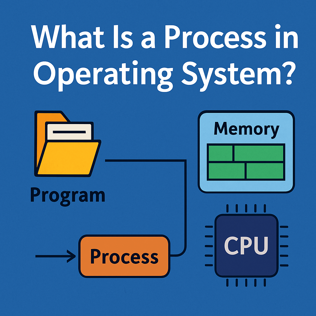
Scheduling in operating systems is like the brain behind all multitasking—it determines which processes get CPU time, in what order, and for how long. Without an efficient scheduler, even the fastest computer would feel sluggish, unresponsive, or chaotic.
In this in-depth, SEO-optimized guide, we’ll dive into:
Fundamental scheduling types and goals
Key metrics for evaluating scheduler efficiency
Popular and advanced scheduling policies with real-world examples
In-depth analysis of modern OS schedulers in Linux, Windows, and macOS
Cutting-edge AI-powered scheduling methods revolutionizing the field
Whether you’re a student preparing for exams, a system architect designing operating systems, or a developer optimizing performance, this is your ultimate scheduling handbook.
Table of Contents
Toggle1. Understanding Scheduling & Its Metrics
What is Scheduling in Operating Systems?
Scheduling is the method by which operating systems decide which process or thread runs at a given time. It ensures maximum utilization of the CPU, fairness across processes, and minimum response times.
Types of Scheduling:
Long-Term Scheduling: Determines which jobs or tasks are admitted into the system for processing.
Short-Term Scheduling: Decides which of the ready-to-execute processes gets the CPU.
Medium-Term Scheduling: Suspends or resumes processes to optimize CPU and memory usage.
Key Scheduling Metrics:
CPU Utilization: Percentage of time the CPU is actively working.
Throughput: Total number of processes completed per unit time.
Turnaround Time: Total time from process submission to completion.
Waiting Time: Time spent in the ready queue.
Response Time: Time from submission until the first output is produced.
Understanding these metrics helps in analyzing which scheduling algorithm suits specific workloads and environments best.

2. Classic Scheduling Policies Explained (With Code Examples)
First Come First Serve (FCFS)
Description: Non-preemptive; processes are executed in the order they arrive.
Pros: Simple to implement.
Cons: Leads to long waiting times and the convoy effect.
Best For: Simple batch systems.
					#include <stdio.h>

int main() {
    int n, i;
    int burst_time[100], waiting_time[100], turnaround_time[100];
    int total_waiting_time = 0, total_turnaround_time = 0;

    printf("Enter the number of processes: ");
    scanf("%d", &n);

    // Input burst times
    printf("Enter burst time for each process:\n");
    for(i = 0; i < n; i++) {
        printf("Process %d: ", i + 1);
        scanf("%d", &burst_time[i]);
    }

    // Calculate waiting time
    waiting_time[0] = 0; // First process has 0 waiting time
    for(i = 1; i < n; i++) {
        waiting_time[i] = waiting_time[i-1] + burst_time[i-1];
    }

    // Calculate turnaround time
    for(i = 0; i < n; i++) {
        turnaround_time[i] = waiting_time[i] + burst_time[i];
    }

    // Display results
    printf("\nProcess\tBurst Time\tWaiting Time\tTurnaround Time\n");
    for(i = 0; i < n; i++) {
        printf("P%d\t%d\t\t%d\t\t%d\n", i+1, burst_time[i], waiting_time[i], turnaround_time[i]);
        total_waiting_time += waiting_time[i];
        total_turnaround_time += turnaround_time[i];
    }

    // Calculate and display averages
    float avg_waiting_time = (float)total_waiting_time / n;
    float avg_turnaround_time = (float)total_turnaround_time / n;

    printf("\nAverage Waiting Time: %.2f\n", avg_waiting_time);
    printf("Average Turnaround Time: %.2f\n", avg_turnaround_time);

    return 0;
}
Sample Output (for 3 processes with burst times: 5, 8, 12)
					Process	Burst Time	Waiting Time	Turnaround Time
P1	    5		    0		        5
P2	    8		    5		        13
P3	    12		    13		        25

Average Waiting Time: 6.00
Average Turnaround Time: 14.33
Shortest Job First (SJF) / Shortest Remaining Time First (SRTF)
Description: Executes the process with the smallest burst time next.
Pros: Optimizes average waiting time.
Cons: May cause starvation.
SRTF: Preemptive version that switches when a shorter job arrives.
Round Robin (RR)
Description: Each process gets a fixed time quantum in cyclic order.
Pros: Fair and simple; ideal for time-sharing systems.
Cons: Frequent context switches if quantum is too small.
					#include <stdio.h>

int main() {
    int n, i, time_quantum, total = 0, x, counter = 0;
    int wait_time = 0, turnaround_time = 0;
    int arrival_time[10], burst_time[10], temp_burst_time[10];

    printf("Enter the total number of processes: ");
    scanf("%d", &n);
    x = n;

    for(i = 0; i < n; i++) {
        printf("\nEnter arrival time of process %d: ", i + 1);
        scanf("%d", &arrival_time[i]);
        printf("Enter burst time of process %d: ", i + 1);
        scanf("%d", &burst_time[i]);
        temp_burst_time[i] = burst_time[i]; // store burst times in temp
    }

    printf("\nEnter the time quantum: ");
    scanf("%d", &time_quantum);

    printf("\nProcess\tBurst Time\tWaiting Time\tTurnaround Time");

    int time = 0;
    for(total = 0, i = 0; x != 0;) {
        if(temp_burst_time[i] > 0 && temp_burst_time[i] <= time_quantum) {
            time += temp_burst_time[i];
            temp_burst_time[i] = 0;
            counter = 1;
        } else if(temp_burst_time[i] > 0) {
            temp_burst_time[i] -= time_quantum;
            time += time_quantum;
        }

        if(temp_burst_time[i] == 0 && counter == 1) {
            x--;
            int wt = time - arrival_time[i] - burst_time[i];
            int tat = time - arrival_time[i];

            printf("\nP%d\t%d\t\t%d\t\t%d", i + 1, burst_time[i], wt, tat);

            wait_time += wt;
            turnaround_time += tat;
            counter = 0;
        }

        // Move to next process
        if(i == n - 1)
            i = 0;
        else if(arrival_time[i + 1] <= time)
            i++;
        else
            i = 0;
    }

    float avg_wait = (float)wait_time / n;
    float avg_turnaround = (float)turnaround_time / n;

    printf("\n\nAverage Waiting Time: %.2f", avg_wait);
    printf("\nAverage Turnaround Time: %.2f\n", avg_turnaround);

    return 0;
}
Priority Scheduling
Description: Each process is assigned a priority; highest priority runs first.
Pros: Suitable for critical systems.
Cons: Lower-priority processes may suffer starvation.
Solution: Aging technique increases the priority of waiting processes over time.
Multilevel and Multilevel Feedback Queue (MLFQ)
Multilevel Queue: Processes are divided into queues based on characteristics (interactive, system, batch).
Multilevel Feedback: Processes can move between queues based on behavior.
Real-World Use: Found in Windows and Unix variants.

3. Inside Modern OS Schedulers
Linux: Completely Fair Scheduler (CFS)
Utilizes a red-black tree data structure to distribute CPU fairly.
Introduced to solve fairness and latency issues.
Tracks virtual runtime to make scheduling decisions.
Linux (2023+): EEVDF Scheduler
Offers latency guarantees while maintaining fairness.
Designed for interactive and real-time workloads.
A major evolution in process scheduling.
Windows Scheduler
Uses Multilevel Feedback Queues with dynamic priority adjustments.
Balances responsiveness and system load using priority boosting and decay.
macOS Scheduler
Based on BSD scheduling with interactivity bias.
Designed for fluid UI/UX with layered priority queues.
Real-Time Scheduling Policies
Rate Monotonic Scheduling (RMS): Fixed priority; shorter periods = higher priority.
Earliest Deadline First (EDF): Dynamic priorities based on deadline proximity.
Both are used in real-time embedded systems.
4. Advanced Scheduling Mechanics
Context Switching
Time required to switch from one process to another.
More switches = higher overhead = lower CPU efficiency.
Preemptive vs Non-Preemptive
Preemptive: Allows interruption for higher-priority processes.
Non-Preemptive: Processes run until they finish or yield control.
CPU Affinity and Load Balancing
Assigns specific processes to specific cores.
Increases cache hit rate and performance in multicore CPUs.
Deadlocks and Starvation
Deadlocks: Circular wait where no process can proceed.
Starvation: Low-priority processes never get CPU.
Solutions include priority aging and deadlock avoidance algorithms.
5. AI-Enhanced Scheduling: The Future Is Here
Reinforcement Learning Schedulers
Algorithms like Q-Learning and Double DQN dynamically learn the best policies based on system state feedback.
Adaptable, self-tuning systems reduce latency and increase throughput in changing workloads.
Semantic Scheduling for LLMs
Prioritizes tasks based on meaning, urgency, and impact.
Useful in AI and NLP workloads where timing affects inference quality.
Predictive Scheduling with LSTM and Neural Networks
Forecasts future CPU and memory needs.
Enables predictive scaling in cloud environments.
Advantages and Trade-offs
Advantages: Efficiency, adaptability, better energy use.
Trade-offs: Computational cost, complexity, unpredictability in real-time environments.
6. Real-World Use Cases, Simulators, and Tools
Popular Tools for Simulation and Testing
htop,top,perf,sched_debugfor LinuxWindows Process Explorer
Web-based OS scheduling simulators
Open Source Projects
Linux Kernel (
kernel/sched/directory)Windows GitHub debugging tools
BPF-based
sched_extcustom schedulers
Hands-On Practice Ideas
Implement your own Round Robin or Priority scheduler in C or Java.
Visualize Gantt charts for multiple algorithms.
Simulate starvation scenarios and apply aging.
Conclusion: Scheduling Smarter in 2025
Scheduling lies at the core of every responsive and efficient system. From classic FCFS and Round Robin to real-time EDF and AI-enhanced strategies like Q-learning, the evolution of schedulers continues to shape the future of computing.
With the rise of cloud computing, real-time analytics, and large language models, smart scheduling is more vital than ever. This guide equips you with the foundational knowledge and future-forward insight to build or optimize any OS-level scheduler.
Next Steps:
Experiment with simulators
Study the Linux kernel’s scheduler
Develop your own predictive or AI-powered scheduler
Monitor real-time behavior using OS performance tools
Frequently Asked Questions (FAQ)
Q1: What is Round Robin Scheduling?
A1: Round Robin Scheduling is a CPU scheduling algorithm where each process is assigned a fixed time quantum in cyclic order. It ensures fair CPU allocation and is widely used in time-sharing systems.
Q2: How does Round Robin differ from First Come First Serve (FCFS)?
A2: Unlike FCFS, which executes processes in the order they arrive without preemption, Round Robin allows each process a limited CPU time slice, then cycles through all processes, preventing any single process from monopolizing the CPU.
Q3: What is a time quantum in Round Robin scheduling?
A3: A time quantum (or time slice) is the fixed amount of CPU time allocated to each process before the scheduler switches to the next process.
Q4: How is waiting time calculated in Round Robin?
A4: Waiting time is the total time a process spends in the ready queue waiting for CPU execution, calculated by subtracting the process’s burst time and arrival time from its finish time.
Q5: Can Round Robin cause high context switching overhead?
A5: Yes, if the time quantum is too small, the CPU frequently switches between processes, leading to increased overhead and reduced efficiency.
Q6: What are the advantages of Round Robin scheduling?
A6: It is simple, fair, and ensures all processes get CPU time regularly, which improves system responsiveness, especially in interactive systems.
Q7: When should Round Robin not be used?
A7: It’s less efficient for processes with varying burst times, especially when short processes are delayed by long ones, and it can cause high overhead if the time quantum is improperly chosen.
Q8: How do modern operating systems implement scheduling?
A8: Modern OSes like Linux use advanced schedulers (e.g., Completely Fair Scheduler – CFS) that blend multiple algorithms and incorporate fairness, interactivity, and real-time constraints.
Q9: What is starvation, and does Round Robin prevent it?
A9: Starvation occurs when a process waits indefinitely due to lower priority. Round Robin’s cyclic approach prevents starvation by giving each process regular CPU access.
Q10: Can AI improve CPU scheduling?
A10: Yes! AI-powered schedulers use machine learning to adaptively optimize scheduling policies based on workload patterns, improving efficiency and responsiveness dynamically.


